38 how to label peaks in excel

Data Smoothing in Excel - dummies The key is to right-click on the plot area and choose Select Data from the pop-up menu. Click on the name of the data series that represents the smoothed line, edit the cell range of the series to reflect the column that holds the particular smoothing technique, and click OK to close the editing dialog boxes. highlighted PEAKS and TROUGHS in a data series in excel In other words, a change of direction is required in order for a number to be considered as a peak or trough. (*** interval between (1). peak to trough 06 hours 13 minutes (approximately). (2). peak (or trough) to peak (trough) 12 hours 26 minutes (approx.)) This thread is locked.

How to Make a Pie Chart in Excel - WinBuzzer Here's how to make one: Select your data, press the pie icon in the "Insert" tab of the ribbon, and click the pie of pie icon A pie of pie chart in Excel is indicated by a picture of a big and...

How to label peaks in excel

How to plot XRD Pattern (Indexing Peaks) using Microsoft ... #XRDPattern #MSExcel Find, label and highlight a certain data point in Excel ... Select the Data Labels box and choose where to position the label. By default, Excel shows one numeric value for the label, y value in our case. To display both x and y values, right-click the label, click Format Data Labels…, select the X Value and Y value boxes, and set the Separator of your choosing: Label the data point by name Finding peaks in Excel data series - Wolfram Research Wolfram Community forum discussion about Finding peaks in Excel data series. Stay on top of important topics and build connections by joining Wolfram Community groups relevant to your interests. ... In Excel 2010 32-bit, suppose I have a data series identified by X (row 1) and Y (row 2):

How to label peaks in excel. Chromatogram in Excel - Chromatography Forum A simple "peak picker" would be to look for the first derivative (essentially the difference between successive measurements) to drop down below zero. You could then in essence query the data for those transition points. It's not going to be as good as a purpose-made data system, but . . . -- Tom Jupille LC Resources / Separation Science Associates How to find peaks and label peaks in origin - YouTube #findpeaksinorigin #labelpeaksinorigin #sayphysics0:00 how to find peaks in origin0:36 how to label peaks in origin 2:32 how to mark peaks in origin4:50 how ... How to Make Your Excel Line Chart Look Better - MBA Excel Under Label Position, Select - Above Input Ctrl + B to make the label bold In the main ribbon, increase label font size to 12 pt. Logic: Within line charts, data labels can be added to all points. However, if we don't want to the chart to become too numbers heavy, we can simply choose to emphasize the peak, trough, or period end of the trend. Label Excel Chart Min and Max • My Online Training Hub Excel Line Chart with Min & Max Markers. Step 1: Insert the chart; select the data in cells B5:E29 > insert a line chart with markers. Step 2: Fix the horizontal axis; right-click the chart > Select Data > Edit the Horizontal (Category) Axis Labels and change the range to reference cells A6:B29. Step 3: Format the markers; click on the max ...

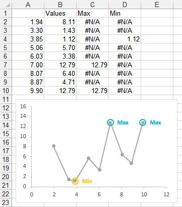
Highlight Minimum and Maximum in an Excel Chart - Peltier Tech Let's do a little formatting. Right click on the Max point, and choose Data Labels. Select the label and choose the Series Name option, so it shows "Max", and choose the bright blue text color. Format the marker so it's an 8-point circle with a 1.5-pt matching blue border and no fill. Right click on the Min point, and choose Data Labels. Highlight High and Low Points in an Excel Chart Dynamically Get your data in place. To highlight the high and low points on the column chart, we need to generate two extra columns of data -one for highest value and the other for the lowest value. The formula used for the minimum column is equally the same with the one shown for the maximum column below. The only difference is that instead of MAX you ... Add a DATA LABEL to ONE POINT on a chart in Excel All the data points will be highlighted. Click again on the single point that you want to add a data label to. Right-click and select ' Add data label '. This is the key step! Right-click again on the data point itself (not the label) and select ' Format data label '. You can now configure the label as required — select the content of ... Automatically place markers on the peaks of a spreadsheet Dim RngLabels As Range, Labels As DataLabels, Ser As Series, I As Long, N As Long, _ StrSer As String Const C As String = "m" If TypeName (Selection) = "Series" Then Set Ser = Selection StrSer = Ser.Formula StrSer = Left (StrSer, InStrRev (StrSer, ",") - 1) StrSer = Right (StrSer, Len (StrSer) - InStrRev (StrSer, ","))

How to count number of peaks in a column of data in Excel? Please do as follows. 1. Select the cell - C3 which is adjacent to cell B3 (the second cell value of your list excluding the header), enter formula =IF (AND (B3>B2,B3>B4), "Peak","") into the Formula Bar and press the Enter key. Then drag the Fill Handle down to mark all peaks as below screenshot shown. 2. Change axis labels in a chart - support.microsoft.com On the Character Spacing tab, choose the spacing options you want. To change the format of numbers on the value axis: Right-click the value axis labels you want to format. Click Format Axis. In the Format Axis pane, click Number. Tip: If you don't see the Number section in the pane, make sure you've selected a value axis (it's usually the ... How to Highlight When Line Drops or Peaks in Comparison Excel Chart Follow these steps: Step 1: Add Three Helper Columns. To make a chart that shades the up and downs of the line in comparison, we will need three helper columns. The first helper column will contain the same values as the first week. I name it week1 shade. In Cell D2, write this formula and drag it down. =B2. Highlight Max & Min Values in an Excel Line Chart - XelPlus Place the data label above the MAX data point by selecting Format Data Labels (right panel) -> expand Label Options -> set the Label Position to Above Since this will always be highest point on the line, it makes sense to display it above the data point. For the MIN data label: Select the MIN data point

32 How To Label Peaks In Excel - Labels Database 2020

How to Add Data Labels to an Excel 2010 Chart - dummies Use the following steps to add data labels to series in a chart: Click anywhere on the chart that you want to modify. On the Chart Tools Layout tab, click the Data Labels button in the Labels group. A menu of data label placement options appears: None: The default choice; it means you don't want to display data labels.

32 How To Label Peaks In Excel - Labels Database 2020

Auto detect and label the peaks and botttoms of a graph? To label the points simply add another data series and apply data labels to it. For any point you don't want displayed use =NA () instead of the data value. Determining which points constitute a peak or a trough may require VBA. Cheers Andy Register To Reply Bookmarks Digg del.icio.us StumbleUpon Google Posting Permissions

Key Features by Version

Excel tutorial: Dynamic min and max data labels To make the formula easy to read and enter, I'll name the sales numbers "amounts". The formula I need is: =IF (C5=MAX (amounts), C5,"") When I copy this formula down the column, only the maximum value is returned. And back in the chart, we now have a data label that shows maximum value. Now I need to extend the formula to handle the minimum value.

32 How To Label Peaks In Excel - Labels Design Ideas 2020

charts - Excel, giving data labels to only the top/bottom ... 1) Create a data set next to your original series column with only the values you want labels for (again, this can be formula driven to only select the top / bottom n values). See column D below. 2) Add this data series to the chart and show the data labels. 3) Set the line color to No Line, so that it does not appear! 4) Volia! See Below! Share

excel - Is it possible to insert text boxes/labels into a chart using ...

Help Online - Tutorials - Picking and Marking Peaks - Origin In the first page (the Start page), select the Find Peaks radio button in the Goal group. Then click the Next button to go to the next page. In the Baseline Mode page, select None (Y=0) for Baseline Mode. Click the Next button to go to the Find Peaks page. In the find Peaks page: Expand the Peak Finding Settings branch.

What Would Earth’s Atmosphere Look Like from the Webb Telescope?

Add or remove data labels in a chart Click Label Options and under Label Contains, select the Values From Cells checkbox. When the Data Label Range dialog box appears, go back to the spreadsheet and select the range for which you want the cell values to display as data labels. When you do that, the selected range will appear in the Data Label Range dialog box. Then click OK.

Is your Outlier Correction outstanding? - APT4 - Outlier CorrectionAPT4

How to add axis label to chart in Excel? - ExtendOffice You can insert the horizontal axis label by clicking Primary Horizontal Axis Title under the Axis Title drop down, then click Title Below Axis, and a text box will appear at the bottom of the chart, then you can edit and input your title as following screenshots shown. 4.

Highlight Minimum and Maximum in an Excel Chart - Peltier Tech

Histogram with Actual Bin Labels Between Bars - Peltier Tech Most histograms made in Excel don't look very good. Partly it's because of the wide gaps between bars in a default Excel column chart. Mostly, though, it's because of the position of category labels in a column chart. The labels are centered below the bars, but it would look nicer with the bin value labels positioned between the bars.

[QUESTION] WithChunkReading not solving memory issues · Issue #2919 ...

Identifying PEAKS and TROUGHS in a data series - MrExcel Message Board If I wanted to calculate " = ceiling (peak_value within the last 30 numbers, 1) - floor (2nd peak_value within the last 30 numbers, 1) ", how should I proceed? Thanks again P PaddyD MrExcel MVP Joined May 1, 2002 Messages 14,234 Aug 20, 2003 #7 ADVERTISEMENT